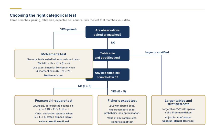
Use Fisher's exact test when expected cell counts fall below 5 in any cell of your contingency table, and use the chi-square test when all expected counts are 5 or higher. That single rule settles the most common decision researchers face when analyzing categorical data. When you are unsure which test fits your design, our statistical test selector points you to the right one. Karl Pearson introduced the chi-square test in 1900 as a goodness-of-fit measure, while Ronald Fisher developed the exact test in 1922 specifically for small-sample contingency tables. Over a century later, these two tests remain the foundation of categorical data analysis in clinical trials, epidemiological studies, and systematic reviews.
| Your data | Test to use |
|---|---|
| All expected cell counts 5 or higher | Chi-square test |
| Any expected cell count below 5 | Fisher's exact test |
| Paired or matched observations | McNemar's test |
| 2x2 tables stratified by a confounder | Cochran-Mantel-Haenszel test |
This guide walks you through every decision point, from hand calculations and continuity corrections to advanced stratified analyses, reporting standards, and R code you can run immediately.
Try our free Chi-Square Calculator to run either test instantly with automatic assumption checking.
Why Expected Cell Counts Drive the Decision
The chi-square test is an asymptotic approximation. It assumes that the sampling distribution of your test statistic follows a chi-square distribution, but this assumption only holds when sample sizes are large enough. The key metric is the expected cell frequency in each cell of your contingency table.
The rule: if any expected cell count is less than 5, switch to Fisher's exact test. To calculate expected counts, multiply each cell's row total by its column total, then divide by the grand total. For a 2x2 table with cells a, b, c, d and row totals R1, R2 and column totals C1, C2, the expected count for cell a equals (R1 x C1) / N.
When expected counts are borderline (between 5 and 10), both tests typically produce similar p-values. The divergence becomes meaningful when expected counts drop below 5, because the chi-square approximation inflates the Type I error rate in that range. Some textbooks use a threshold of 10 instead of 5, but the widely accepted convention in biomedical research is 5.
Step-by-Step Calculation Example with Real Clinical Data
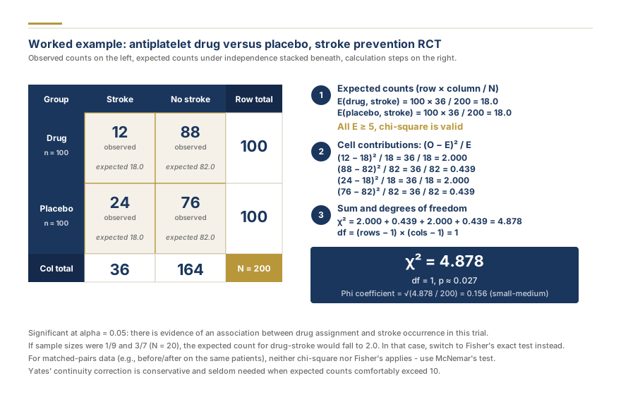
Consider a randomized controlled trial comparing a new antiplatelet drug to placebo for preventing stroke. The 2x2 contingency table:
| Stroke | No Stroke | Row Total | |
|---|---|---|---|
| Drug | 12 | 88 | 100 |
| Placebo | 24 | 76 | 100 |
| Column Total | 36 | 164 | 200 |
Step 1: Calculate expected cell counts.
- Expected (Drug, Stroke) = (100 x 36) / 200 = 18.0
- Expected (Drug, No Stroke) = (100 x 164) / 200 = 82.0
- Expected (Placebo, Stroke) = (100 x 36) / 200 = 18.0
- Expected (Placebo, No Stroke) = (100 x 164) / 200 = 82.0
All expected counts exceed 5, so the chi-square test is appropriate here.
Step 2: Compute the chi-square statistic.
For each cell, calculate (Observed - Expected)^2 / Expected:
- (12 - 18)^2 / 18 = 36 / 18 = 2.00
- (88 - 82)^2 / 82 = 36 / 82 = 0.439
- (24 - 18)^2 / 18 = 36 / 18 = 2.00
- (76 - 82)^2 / 82 = 36 / 82 = 0.439
Chi-square statistic = 2.00 + 0.439 + 2.00 + 0.439 = 4.878
Step 3: Determine the p-value.
With 1 degree of freedom (df = (rows - 1) x (cols - 1) = 1), the p-value for a chi-square of 4.878 is approximately 0.027. This is below the conventional alpha of 0.05, suggesting a statistically significant association between drug assignment and stroke occurrence.
Step 4: Calculate the effect size.
The phi coefficient = sqrt(4.878 / 200) = sqrt(0.02439) = 0.156, indicating a small-to-medium effect. You can compute this instantly using our effect size estimator.
Now imagine the same proportions but with a total sample of only 20 patients (Drug: 1 stroke, 9 no stroke; Placebo: 3 strokes, 7 no stroke). The expected count for the Drug/Stroke cell would be (10 x 4) / 20 = 2.0, which falls below 5. In that scenario, you would use Fisher's exact test instead.
Fisher's Exact Test
Fisher's exact test calculates the exact probability of observing your data (or a more extreme result) given the null hypothesis of no association. It does not rely on an approximation, which is why it remains valid regardless of sample size. Fisher developed this approach using the hypergeometric distribution, which models the probability of each possible 2x2 table configuration given fixed row and column totals.
For the small-sample stroke example above (1, 9, 3, 7 with N = 20), Fisher's exact test would enumerate all possible tables with those marginals and sum the probabilities of tables as extreme or more extreme than the observed one. The resulting two-sided p-value would be approximately 0.582, indicating no significant association. This contrasts sharply with what a naive chi-square application would suggest, demonstrating why test selection matters.
Fisher's exact test is primarily designed for 2x2 tables. For larger tables, the Freeman-Halton test generalizes the logic, though computation becomes intensive as table dimensions grow.
Chi-Square with Yates' Continuity Correction
Frank Yates introduced his continuity correction in 1934 to bridge the gap between the discrete chi-square test statistic and the continuous chi-square distribution. The correction subtracts 0.5 from the absolute difference between observed and expected counts before squaring:
Corrected chi-square = Sum of (|Observed - Expected| - 0.5)^2 / Expected
For our stroke example, the corrected statistic would be:
- (|12 - 18| - 0.5)^2 / 18 = (5.5)^2 / 18 = 1.681
- And similarly for the other three cells.
The corrected chi-square = 4.167, yielding p = 0.041 (compared to p = 0.027 without correction).
When to apply Yates' correction:
- Only for 2x2 tables (never for larger contingency tables)
- When expected counts are between 5 and 10 in one or more cells
- When you want a conservative estimate that approximates the two-sided Fisher's exact p-value
When to skip it:
- When all expected counts comfortably exceed 10
- When you already plan to use Fisher's exact test for small samples
- When journal guidelines or reviewers specifically request the uncorrected version
Many modern statisticians, including those publishing simulation studies in Statistics in Medicine and the British Medical Journal, now consider Yates' correction overly conservative for routine use. It reduces statistical power, potentially masking genuine effects. The safest approach: if expected counts are borderline, skip the correction and run Fisher's exact test directly.
McNemar's Test for Paired and Matched Data
Neither the chi-square test nor Fisher's exact test is appropriate when your categorical observations are paired or matched. Consider a before-and-after study where the same 80 patients are tested for antibiotic resistance before and after treatment:
| After: Resistant | After: Susceptible | |
|---|---|---|
| Before: Resistant | 10 (a) | 25 (b) |
| Before: Susceptible | 5 (c) | 40 (d) |
The standard chi-square test would treat these 80 paired observations as if they were 80 independent observations, violating the independence assumption. McNemar's test focuses only on the discordant pairs (cells b and c), where change actually occurred.
McNemar's test statistic = (b - c)^2 / (b + c) = (25 - 5)^2 / (25 + 5) = 400 / 30 = 13.33
With 1 degree of freedom, this yields p < 0.001, indicating a significant change in resistance patterns after treatment.
When the number of discordant pairs (b + c) is small (below 25), use the exact binomial version of McNemar's test instead of the chi-square approximation.
Common scenarios requiring McNemar's test in clinical research include pre-post intervention studies, matched case-control designs, and diagnostic test comparisons where the same patients undergo two different tests.
Cochran-Mantel-Haenszel Test for Stratified Tables
When you need to test an association while controlling for a confounding variable, the Cochran-Mantel-Haenszel (CMH) test is the standard approach. William Cochran proposed the method in 1954, and Nathan Mantel and William Haenszel extended it in 1959 for case-control studies.
Imagine testing whether a drug reduces infection across three hospitals. Each hospital produces a separate 2x2 table, and infection rates differ by hospital (a confounding variable). The CMH test combines evidence across all strata (hospitals) to produce a single pooled test of association while adjusting for the stratifying variable.
The CMH statistic follows a chi-square distribution with 1 degree of freedom under the null hypothesis of no association across strata. It also produces a common odds ratio (the Mantel-Haenszel odds ratio), which is the weighted average of stratum-specific odds ratios.
When to use CMH:
- Multicenter clinical trials with center as a stratifying variable
- Studies adjusting for a categorical confounder (age group, sex, disease severity)
- Systematic reviews combining 2x2 tables across studies (this is essentially what a fixed-effect meta-analysis does with the Mantel-Haenszel method)
The CMH test assumes a consistent direction of association across strata (no qualitative interaction). Test this assumption with the Breslow-Day test for homogeneity of odds ratios before interpreting the CMH result.
For researchers conducting systematic reviews and meta-analyses, understanding the CMH framework is essential because the Mantel-Haenszel method is one of the two primary approaches (alongside inverse-variance) for pooling binary outcome data. Learn more about choosing the right statistical test for your research.
Larger Contingency Tables: 3x2, 4x2, and Beyond
The chi-square test generalizes naturally to tables larger than 2x2. A 3x2 table (3 exposure groups, 2 outcomes) has (3 - 1) x (2 - 1) = 2 degrees of freedom. A 4x3 table has 6 degrees of freedom.
For these larger tables, the expected count rule still applies: if more than 20% of cells have expected counts below 5, or if any cell has an expected count below 1, the chi-square approximation becomes unreliable.
Fisher's exact test becomes computationally impractical for larger tables because the number of possible configurations grows exponentially. A 2x2 table with N = 20 might have a few dozen possible configurations. A 4x5 table with N = 200 could have millions. For these situations, Monte Carlo simulation provides the solution: randomly generate thousands (typically 10,000 or more) of tables with the same marginals, compute the test statistic for each, and estimate the p-value from the empirical distribution.
Practical guidance for larger tables:
| Table Size | Expected Counts OK | Expected Counts Low |
|---|---|---|
| 2x2 | Chi-square | Fisher's exact |
| 3x2 or 2x3 | Chi-square | Fisher-Freeman-Halton or Monte Carlo |
| 4x2 or larger | Chi-square | Monte Carlo simulation (B = 10,000+) |
| Any with ordinal outcome | Chi-square for trend | Exact trend test |
When your variable is ordinal (e.g., disease severity: mild, moderate, severe), a chi-square test for linear trend (also called the Cochran-Armitage test) is more powerful than the standard chi-square test because it exploits the ordering information.
Harald Cramer introduced Cramer's V in 1946 as the standard effect size measure for tables larger than 2x2. For a table with r rows and c columns, Cramer's V = sqrt(chi-square / (N x min(r - 1, c - 1))). Benchmarks for Cramer's V depend on the smaller dimension: for df* = 1, small = 0.10, medium = 0.30, large = 0.50; for df* = 2, small = 0.07, medium = 0.21, large = 0.35.
Exact vs. Asymptotic P-Values: What the Difference Means Clinically
The distinction between exact p-values and asymptotic p-values often confuses researchers, but it has real clinical implications.
An asymptotic p-value comes from the chi-square distribution, which is a theoretical distribution that the test statistic approaches as sample size grows toward infinity. For large samples, this approximation is excellent. For small samples, it can be inaccurate in either direction.
An exact p-value is calculated by enumerating all possible data configurations and summing their probabilities. It makes no distributional assumptions and is always valid, regardless of sample size.
When do they diverge clinically?
Consider a small pilot study (N = 30) that produces a chi-square p-value of 0.042 and a Fisher's exact p-value of 0.071. The chi-square result would lead you to reject the null hypothesis, while Fisher's exact test would not. This discrepancy could determine whether a pilot study proceeds to a full-scale trial, influencing thousands of future patients.
In regulatory submissions and clinical trial reports, the FDA and EMA both accept Fisher's exact test for small samples. Many journal guidelines (including CONSORT for randomized trials) recommend reporting the exact p-value when sample sizes are small. If both tests agree (both significant or both non-significant), report either one. If they disagree, report Fisher's exact test and note the discrepancy.
For a deeper understanding of p-values in the context of research synthesis, see our guide on p-values and confidence intervals explained.
How to Report Chi-Square and Fisher's Results in a Manuscript
Want to run your own 2x2 table? Use our chi-square calculator with APA-formatted results, or the Fisher's exact test calculator when expected counts fall below 5. Both export a written results paragraph in APA 7 style.
Clear reporting is essential for reproducibility. Follow these APA-style reporting formats:
Chi-square test: "A chi-square test of independence was performed to examine the relationship between treatment group and stroke occurrence. The association was statistically significant, chi-square(1, N = 200) = 4.88, p = .027, phi = 0.16."
Chi-square with Yates' correction: "With Yates' continuity correction, the association remained significant, chi-square(1, N = 200) = 4.17, p = .041, phi = 0.16."
Fisher's exact test: "Because two cells had expected counts below 5, Fisher's exact test was used. The association between treatment and outcome was not statistically significant (p = .582, two-tailed)."
McNemar's test: "McNemar's test indicated a significant change in antibiotic resistance after treatment, chi-square(1) = 13.33, p < .001."
Key reporting elements to include every time:
- The test name and why it was chosen (especially for Fisher's exact test)
- Degrees of freedom and sample size for chi-square
- The exact p-value (not just "p < 0.05")
- An effect size measure (phi for 2x2, Cramer's V for larger tables)
- Whether the test was one-tailed or two-tailed
Reviewers frequently reject manuscripts that report chi-square results without effect sizes. Always pair your statistical significance with a measure of practical significance.
Need help with the statistical analysis section of your manuscript? Our biostatisticians handle everything from test selection to APA-formatted results tables. Request a free quote and tell us about your project.
Using Chi-Square Results in Meta-Analysis
When conducting a meta-analysis of studies reporting binary outcomes, you often encounter studies that report only a chi-square statistic or a p-value rather than a full 2x2 table. Converting these values to effect sizes suitable for pooling requires a few steps.
Converting chi-square to an odds ratio:
For a 2x2 table, you can recover the log odds ratio from the chi-square statistic if you also know the marginal totals. If only the chi-square and N are available, you can approximate:
- phi = sqrt(chi-square / N)
- For a 2x2 table with balanced groups: OR is approximately exp(phi x pi / sqrt(3))
However, this approximation is rough. Whenever possible, extract or reconstruct the full 2x2 table from the original paper. Contact study authors if the table is not reported.
Converting a p-value to a test statistic:
If a study reports only "p = 0.03" for a chi-square test with 1 df, you can recover the chi-square statistic using the inverse chi-square distribution. In R: qchisq(1 - 0.03, df = 1) gives approximately 4.71.
Why this matters for systematic reviews:
In a systematic review, inconsistent test reporting across primary studies is one of the biggest obstacles to quantitative synthesis. Some studies report Fisher's exact p-values, others report chi-square statistics, and some report only odds ratios with confidence intervals. Understanding the relationship between these quantities lets you convert between formats and include more studies in your meta-analysis, increasing statistical power.
For converting between effect size formats, use our Cohen's d calculator.