Converting Effect Sizes: Cohen's d to Hedges g

When you pool results across studies in a meta-analysis, you will almost certainly face a common problem: different studies report different effect sizes. One trial reports an odds ratio (OR), another reports a standardized mean difference (SMD), and a third gives you a Cohen's d. Before you can run a pooled analysis, everything must be on the same scale.

This guide walks you through every common conversion formula, explains when each effect size is appropriate, provides worked examples with real numbers, and covers practical issues like missing data, software implementation in R, and reporting requirements for journals and reviewers.

Try our free online effect size tool to run these conversions without manual computation.

Choosing the Right Effect Size for Your Data

Cohen's d is the most familiar standardized mean difference. It divides the difference between two means by a pooled standard deviation. It works well when sample sizes are reasonably large (typically above 20 per group). Cohen (1988) introduced the metric along with the widely cited benchmarks of 0.2, 0.5, and 0.8 for small, medium, and large effects in behavioral research.

Hedges' g is a corrected version of Cohen's d. When sample sizes are small, Cohen's d systematically overestimates the true effect size. Hedges (1981) introduced a correction factor (sometimes called J) that removes this small-sample bias. In most meta-analyses, Hedges' g is the preferred choice, and it is the default in the metafor R package developed by Viechtbauer (2010).

The odds ratio is used for binary outcomes. It expresses how much more likely the event is in one group compared to another. The Cochrane Handbook recommends the odds ratio for meta-analyses of clinical trials with dichotomous outcomes because it has desirable mathematical properties, including symmetry around the null.

The risk ratio (RR), also called the relative risk, is also for binary outcomes but is more intuitive for clinical interpretation. Clinicians often prefer risk ratios in treatment guidelines because they communicate the magnitude of benefit more directly than odds ratios.

The Pearson correlation coefficient (r) is a standardized measure of linear association between two continuous variables. It ranges from -1 to +1 and is commonly reported in observational studies and psychometric research.

The number needed to treat (NNT) is derived from the absolute risk difference. You can use our free NNT Calculator to move between risk difference and NNT.

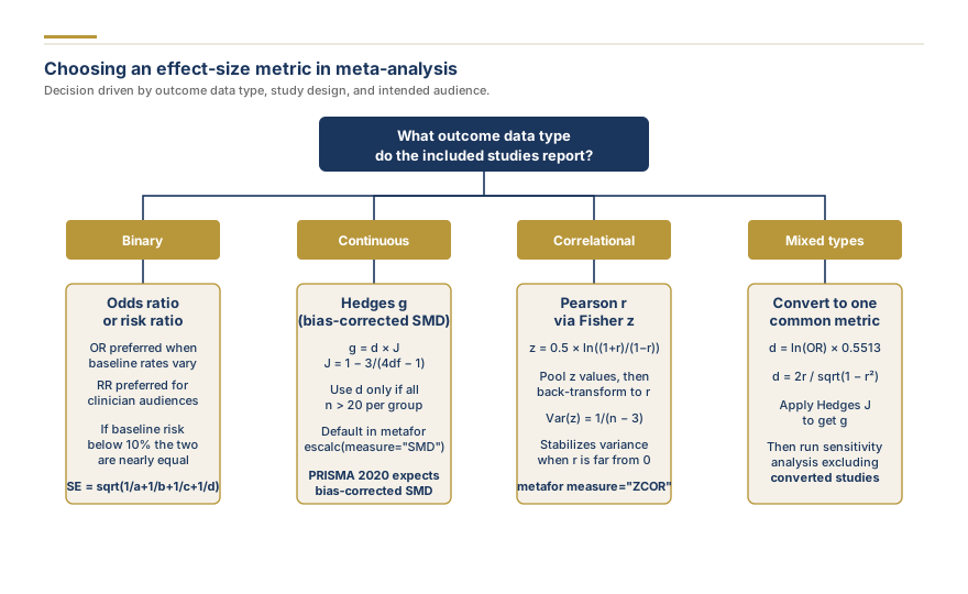
When to Use Each Effect Size Metric: A Decision Flowchart

Choosing the right metric depends on three factors: the type of outcome data, the design of included studies, and the intended audience of your findings.

Binary outcomes (yes/no events). If all studies report event counts, use the odds ratio or risk ratio directly. The odds ratio is preferred when baseline event rates vary substantially across studies. The risk ratio is preferred when your audience is clinicians who need intuitive interpretation. If baseline risk is below 10%, the two metrics produce nearly identical results.

Continuous outcomes. If all studies report means and standard deviations for two groups, compute Hedges' g (corrected standardized mean difference). Use Cohen's d only if you have a specific reason and all sample sizes exceed 20 per group.

Correlational data. If studies report associations between two continuous variables, use Pearson r or convert to Fisher's z for pooling. Fisher's z transformation stabilizes the variance when correlations are far from zero.

Mixed outcome types. This is the most complex scenario. When some studies report binary outcomes (odds ratios) and others report continuous outcomes (mean differences), you must convert everything to a single metric. The standard approach, described by Borenstein et al. (2009), is to convert odds ratios to Cohen's d (or vice versa) using the formulas in this guide. Then apply the Hedges' g correction if needed.

Why Hedges' g Corrects Small-Sample Bias

Cohen's d is calculated as: d = (M1 - M2) / SD_pooled

Hedges' g applies a multiplicative correction factor J: g = d * J

Where J is approximated as: J = 1 - (3 / (4*df - 1)) and df = n1 + n2 - 2.

For large samples (n > 20 per group), J is very close to 1. For small samples (n = 5 per group), J can be around 0.88, meaning d overestimates the true effect by about 12%.

Worked example with real numbers. Suppose a study with n1 = 8 and n2 = 10 reports M1 = 24.3, M2 = 20.1, SD_pooled = 5.6. Cohen's d = (24.3 - 20.1) / 5.6 = 0.750. The degrees of freedom are 8 + 10 - 2 = 16. J = 1 - (3 / (4*16 - 1)) = 1 - (3/63) = 0.952. Hedges' g = 0.750 * 0.952 = 0.714. The correction shaved off about 5% of the effect, which matters when you pool many small studies.

Rule of thumb: Use Hedges' g by default in meta-analyses. The Cochrane Handbook and the PRISMA 2020 reporting guidelines both expect standardized mean differences to be bias-corrected.

Converting Between Effect Sizes: The Formulas

Cohen's d to Hedges' g

g = d * [1 - (3 / (4*(n1+n2-2) - 1))]

Worked example: d = 0.62, n1 = 15, n2 = 18. df = 31. J = 1 - (3 / (4*31 - 1)) = 1 - (3/123) = 0.976. g = 0.62 * 0.976 = 0.605.

Odds Ratio to Cohen's d

The standard formula from Hasselblad and Hedges (1995), widely endorsed by Borenstein et al. (2009): d = ln(OR) * (sqrt(3) / pi), which simplifies to d = ln(OR) * 0.5513

Worked example: An OR of 2.5 gives: ln(2.5) = 0.916, d = 0.916 * 0.5513 = 0.505. So OR = 2.5 corresponds to approximately d = 0.50, a medium effect.

The variance of d converted from an OR is: Var(d) = Var(ln(OR)) * (3 / pi^2). You need this variance for the inverse-variance weighting in your meta-analysis.

Cohen's d to Odds Ratio

OR = exp(d * pi / sqrt(3)) = exp(d * 1.8138)

Worked example: d = 0.40, OR = exp(0.40 * 1.8138) = exp(0.726) = 2.066. A "small-to-medium" standardized mean difference corresponds to roughly doubling the odds.

Risk Ratio to Odds Ratio

When you have a risk ratio and need an OR, you need the baseline risk (p0): OR = RR * (1 - p0) / (1 - RR * p0)

When baseline risk is low (below 10%), OR and RR are approximately equal.

Worked example: RR = 1.8, baseline risk p0 = 0.30. OR = 1.8 * (1 - 0.30) / (1 - 1.8 * 0.30) = 1.8 * 0.70 / (1 - 0.54) = 1.26 / 0.46 = 2.739. Notice how the OR (2.74) is substantially larger than the RR (1.80) when baseline risk is 30%. This is why conflating the two metrics leads to overestimation.

Log Odds Ratio Conversions

Many meta-analysis software packages work on the log odds ratio (ln(OR)) scale because it has better statistical properties: the sampling distribution is approximately normal, and the confidence interval is symmetric.

OR to log OR: ln(OR) = natural logarithm of the odds ratio. Example: OR = 3.2, ln(OR) = 1.163.

Log OR to OR: OR = exp(ln(OR)). Example: ln(OR) = -0.45, OR = exp(-0.45) = 0.638.

Log OR to Cohen's d: d = ln(OR) * 0.5513. This is identical to the OR-to-d formula because d = ln(OR) * (sqrt(3)/pi).

Standard error of log OR: SE(ln(OR)) = sqrt(1/a + 1/b + 1/c + 1/d), where a, b, c, d are the cells of the 2x2 table.

Pearson Correlation (r) to Cohen's d

The correlation coefficient r is common in observational studies and psychometric research. Converting between r and d is essential when your meta-analysis includes both experimental and correlational studies.

r to d: d = 2r / sqrt(1 - r^2)

Worked example: r = 0.35. d = 2(0.35) / sqrt(1 - 0.1225) = 0.70 / sqrt(0.8775) = 0.70 / 0.937 = 0.747.

d to r: r = d / sqrt(d^2 + 4)

Worked example: d = 0.50. r = 0.50 / sqrt(0.25 + 4) = 0.50 / sqrt(4.25) = 0.50 / 2.062 = 0.243.

Use our free Correlation and Effect Size Converter to run these calculations instantly.

Fisher's z transformation. When pooling correlations in a meta-analysis, first transform each r to Fisher's z: z = 0.5 * ln((1+r)/(1-r)). Pool the z values, then back-transform the pooled z to r. This is necessary because the variance of r depends on the population correlation, while the variance of Fisher's z is approximately 1/(n-3) regardless of the correlation magnitude.

Benchmarks and Interpretation

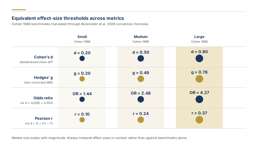
Cohen's (1988) benchmarks: Small (d = 0.2), Medium (d = 0.5), Large (d = 0.8). These were intended as rough guides for psychology research, not universal standards. Always interpret effect sizes in context.

Equivalent benchmarks across metrics:

These cross-metric benchmarks help reviewers quickly calibrate effect sizes reported on unfamiliar scales. The conversions in the table use the formulas from this guide.

For visual pooling and forest plot generation, try our free Forest Plot Generator.

Effect Size Conversion in Meta-Analysis Software

Using escalc() in the metafor Package

The metafor package in R, developed by Viechtbauer (2010), is the most widely used tool for meta-analysis. Its escalc() function handles effect size computation and conversion automatically.

Computing Hedges' g from means and SDs:

library(metafor)

# Two-group comparison data
dat <- data.frame(
  study = c("Smith 2019", "Jones 2020", "Lee 2021"),
  m1 = c(24.3, 18.7, 31.2),
  m2 = c(20.1, 16.9, 27.8),
  sd1 = c(5.6, 4.2, 6.1),
  sd2 = c(5.8, 4.5, 5.9),
  n1 = c(45, 32, 28),
  n2 = c(42, 35, 30)
)

# Compute Hedges' g (measure = "SMD" uses Hedges' g by default)
dat <- escalc(measure = "SMD",
              m1i = m1, m2i = m2,
              sd1i = sd1, sd2i = sd2,
              n1i = n1, n2i = n2,
              data = dat)

Computing log odds ratios from 2x2 tables:

dat_binary <- data.frame(
  study = c("Trial A", "Trial B"),
  ai = c(28, 15),  # events in treatment
  bi = c(72, 85),  # non-events in treatment
  ci = c(42, 22),  # events in control
  di = c(58, 78)   # non-events in control
)

dat_binary <- escalc(measure = "OR",
                     ai = ai, bi = bi,
                     ci = ci, di = di,
                     data = dat_binary)

The escalc() function supports over 60 effect size measures, including "SMD" (Hedges' g), "OR" (log odds ratio), "RR" (log risk ratio), "COR" (raw correlation), and "ZCOR" (Fisher's z-transformed correlation).

Converting between metrics in metafor. If you have a mix of odds ratios and standardized mean differences, convert the odds ratios to SMD first, then combine: compute log(OR), multiply by 0.5513 to get d, apply the Hedges correction, and compute the appropriate variance. Borenstein et al. (2009) provide the variance formulas in Chapter 7 of their textbook.

How to Handle Missing Data for Effect Size Calculation

Real-world studies frequently omit the exact statistics you need. Here are practical strategies for recovering effect sizes from incomplete reporting.

When only t-values or F-values are reported. Convert t to d: d = 2t / sqrt(df). For a one-way ANOVA F with two groups: d = 2 * sqrt(F/df_error). This is exact, not an approximation.

When only p-values are reported. Convert the p-value to a t-statistic using the inverse-t distribution, then convert t to d. This works best when the exact p-value is given (e.g., p = 0.023), not just an inequality (p < 0.05). For inequalities, you can compute a conservative estimate using the boundary value (e.g., t corresponding to p = 0.05).

When only confidence intervals are reported. If a study reports a mean difference with a 95% confidence interval, recover the standard error: SE = (upper - lower) / (2 * 1.96). Then compute d from the mean difference divided by the pooled SD, which you can estimate from the SE and sample sizes.

When medians and interquartile ranges are reported. Use the methods of Wan et al. (2014) or Luo et al. (2018) to estimate the mean and SD from the median, IQR, and sample size. These methods are implemented in the estmeansd R package.

When only event rates (percentages) are reported without raw counts. Multiply the percentage by the group sample size to recover the count. If sample sizes are missing, you may need to contact the original authors or exclude the study.

Documentation is critical. For every imputed or converted effect size, record the method used in a supplementary table. Reviewers and editors expect transparency about how each study's data entered your meta-analysis.

Struggling with effect size conversions or missing data in your meta-analysis? Our biostatisticians handle the entire statistical pipeline, from data extraction through final forest plots. send us your project details and let our team at Research Gold meta-analysis services take the complexity off your plate.

Reporting Effect Sizes in Your Manuscript

APA Style Requirements

The American Psychological Association (APA 7th edition) requires that all quantitative results include effect sizes and their confidence intervals. Specifically:

• Report the type of effect size (e.g., "Hedges' g" not just "effect size" or "ES").
• Include the 95% confidence interval in square brackets: g = 0.52, 95% CI [0.31, 0.73].
• State the direction of the effect explicitly in the text.
• For odds ratios, report on the original scale (not log-transformed) with the confidence interval: OR = 2.48, 95% CI [1.65, 3.73].

PRISMA 2020 Reporting Requirements

The PRISMA 2020 checklist (Item 13a) requires authors to specify "for each synthesis, the effect measure(s) used." This means you must:

• Name the effect size metric in the Methods section (e.g., "We used Hedges' g for continuous outcomes and log odds ratios for binary outcomes").
• Describe any conversions performed (e.g., "Odds ratios were converted to standardized mean differences using the formula of Borenstein et al. (2009) to enable pooling across outcome types").
• Justify the choice of metric with a citation.
• Report the software and version used for computation (e.g., "Effect sizes were computed using the escalc() function in the metafor package version 4.4-0 in R").

Formatting Effect Size Tables

Include a table listing each study's effect size, confidence interval, weight, and the original metric reported by the study authors. If you converted any study's metric, flag it with a footnote explaining the conversion method. This level of detail satisfies the Cochrane Handbook's recommendation for full transparency.

Common Reviewer Questions About Effect Size Choice

Peer reviewers frequently raise questions about effect size decisions. Here are the most common concerns and how to address them.

"Why did you use Hedges' g instead of Cohen's d?" Explain that Hedges' g corrects for the upward bias in Cohen's d when sample sizes are small (Hedges, 1981). Since meta-analyses often include studies with small samples, Hedges' g is the standard recommendation from both the Cochrane Handbook and Borenstein et al. (2009).

"Why did you convert odds ratios to standardized mean differences?" This is appropriate when most of your studies report continuous outcomes but a few report dichotomous outcomes created by dichotomizing an underlying continuous variable. Cite Borenstein et al. (2009), Chapter 7, and explain that the conversion assumes a logistic distribution for the underlying continuous variable.

"How sensitive are your results to the conversion formulas?" Run a sensitivity analysis excluding the converted studies. If the pooled effect does not change meaningfully, state this explicitly. If it does change, discuss the implications. Use our guide on effect size calculation in meta-analysis for additional context on sensitivity approaches.

"Why didn't you use the risk ratio instead of the odds ratio?" The odds ratio has better mathematical properties for meta-analysis: it is unbounded, symmetric on the log scale, and can be estimated from case-control studies. However, if your audience is primarily clinicians, consider reporting both metrics. Convert the pooled OR back to a RR using the baseline risk from the control group of a representative study.

"Can you report NNT alongside the pooled effect?" Yes. Convert the pooled SMD or OR to an NNT using the control group event rate. Report the NNT with a confidence interval. This makes results immediately actionable for clinical decision-makers.

Common Mistakes When Converting Effect Sizes

Using OR as if it were RR. When baseline risk is above 20%, treating an OR as an RR leads to substantial overestimation. A study with OR = 3.0 and baseline risk of 40% corresponds to RR = 1.88, not 3.0.

Ignoring direction. An OR below 1 means the event is less likely in the treatment group. A negative log produces a negative d. Always maintain a consistent direction across all studies in your meta-analysis.

Forgetting sample sizes for the J correction. If you convert d to g without the correct sample sizes, your correction will be wrong. Always extract both n1 and n2 from the original study.

Mixing continuous and binary outcomes without justification. Converting OR to d is appropriate when the underlying construct is continuous and the binary outcome was created by dichotomizing a latent variable. It is not appropriate when the binary outcome is a truly discrete event (e.g., mortality).

Pooling r values directly without Fisher's z transformation. The variance of Pearson r depends on the population correlation, which violates the assumption of known sampling variance in standard meta-analysis models. Always transform to Fisher's z before pooling, then back-transform.

Using Cohen's benchmarks as absolute thresholds. A d of 0.15 in a public health intervention affecting millions of people may be far more consequential than a d of 0.90 in a laboratory experiment with 20 participants. Context determines importance, not arbitrary cutoffs.

Double-correcting for small-sample bias. Some software applies the Hedges correction automatically. If you manually apply J to a value that was already corrected, you will over-correct. Check your software documentation.

Key Takeaways

• Use Hedges' g instead of Cohen's d in meta-analyses, especially when any included studies have small samples (Hedges, 1981).
• Convert odds ratios to Cohen's d using the formula: d = ln(OR) * 0.5513, following Borenstein et al. (2009).
• Convert Pearson r to Cohen's d using: d = 2r / sqrt(1 - r^2), and back with: r = d / sqrt(d^2 + 4).
• When converting between OR and RR, you must know the baseline event rate in the control group.
• Use the escalc() function in the metafor package to automate conversions and variance calculations.
• When data are missing, recover effect sizes from t-values, F-values, p-values, or confidence intervals before excluding a study.
• Report effect sizes following APA 7th edition and PRISMA 2020 guidelines, including the metric name, confidence interval, and any conversion methods used.
• Cohen's benchmarks (0.2, 0.5, 0.8) are starting points, not universal rules. Interpret in context.
• Always track the direction (sign) of effects when converting.
• Run a sensitivity analysis excluding converted studies to address reviewer concerns about formula assumptions.
• Use our effect size estimator and Correlation Effect Size Converter to reduce arithmetic errors in conversion chains.

Need expert help with your systematic review or meta-analysis? Our biostatistics team specializes in complex effect size conversions, multi-format pooling, and publication-ready reporting. Get a free quote today.