High I-squared values are one of the most common problems researchers face when synthesizing evidence. A standard forest plot tells you that heterogeneity is present but not which specific studies are driving it or whether those studies are also distorting your pooled estimate. That is where the Galbraith plot and the Baujat plot become essential.
These two diagnostic plots are available as dedicated tabs inside our free build a forest plot. This guide explains exactly what each plot shows, how to read the output, and how to use the findings to make defensible decisions about your meta-analysis model.
Why Standard Forest Plots Miss the Source of Heterogeneity
A forest plot orders studies vertically and shows each one's confidence interval relative to the null. You can visually detect heterogeneity when the squares are spread widely, but the plot does not distinguish between two fundamentally different situations.
In the first situation, a small number of outlier studies sit far from the rest while the majority of studies cluster tightly. Removing or down-weighting these outliers would substantially reduce I-squared without changing the direction of your overall conclusion.
In the second situation, heterogeneity is diffuse and no single study is responsible. Here, subgroup analysis or meta-regression is the appropriate next step because there is no outlier to remove.
Acting on the wrong diagnosis wastes time and introduces bias. The Galbraith and Baujat plots give you the evidence to distinguish between these two situations before you decide how to proceed.
The Galbraith Plot (Radial Plot): Detecting Outliers by Precision
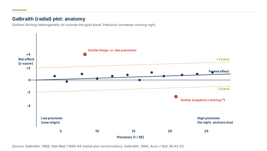
The Galbraith plot, also called a radial plot after its creator Robert Galbraith, was developed specifically to visualize heterogeneity in a way that separates imprecise studies from true outliers.
How it is constructed. Each study is plotted as a single point. The x-axis is the reciprocal of the study's standard error (1/SE), which represents precision: studies with larger samples and smaller standard errors appear further to the right. The y-axis is the study's z-score divided by its standard error (the standardized effect). A regression line is drawn through the origin with a slope equal to the pooled effect estimate. Two outer lines parallel to this regression line mark the boundaries at plus and minus two standard deviations.
What the position means. Studies that fall within the two outer lines are consistent with the pooled estimate. Studies that fall outside these lines are statistical outliers. Critically, because the x-axis encodes precision, you can immediately see whether the outliers are small imprecise studies (clustered near the origin) or large precise studies (far to the right). A large, precise study that is an outlier is far more concerning than a small imprecise one, because it carries more weight in the pooled estimate.
A worked interpretation example. Suppose your meta-analysis has I-squared of 72% and 14 studies. You open the Galbraith plot and see that 12 studies cluster tightly near the regression line while 2 studies sit outside the upper boundary, both positioned at mid-range precision. This pattern suggests localized heterogeneity. You examine those 2 studies in detail, find they used a different comparator intervention, and run a subgroup analysis separating them from the rest. I-squared in the main subgroup drops to 18%.
Common misreading to avoid. Do not treat every point outside the boundary lines as a study to exclude. The two-SD boundary is a statistical flag, not a clinical judgment. Always examine why a study is an outlier before deciding how to handle it.
The Baujat Plot: Separating Heterogeneity Contribution from Influence
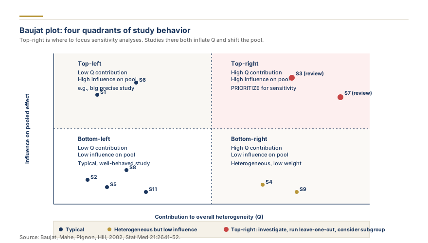
The Baujat plot, developed by Baujat and colleagues in 2002, adds a second dimension that the Galbraith plot does not capture. While the Galbraith plot identifies outliers in terms of effect size, the Baujat plot simultaneously measures two distinct concepts: how much each study contributes to overall heterogeneity, and how much each study influences the pooled estimate.
How it is constructed. The x-axis shows each study's contribution to the overall Q statistic, which is the raw measure of heterogeneity. The y-axis shows the influence of each study on the pooled effect, measured as the squared difference between the overall pooled estimate and the pooled estimate calculated when that study is left out.
Quadrant interpretation. The Baujat plot naturally divides into four quadrants around the median values of each axis.
Studies in the upper-right quadrant contribute heavily to both heterogeneity and influence. These are your priority studies for investigation. They are making your I-squared high and they are moving your pooled estimate significantly. If any single study belongs in this quadrant, examine its methods, population, risk of bias, and publication context carefully.
Studies in the lower-right quadrant contribute to heterogeneity but do not strongly influence the pooled estimate. These studies have unusual effect sizes compared to the rest but carry less weight. Their presence inflates I-squared without necessarily biasing your summary estimate.
Studies in the upper-left quadrant are highly influential but not strong contributors to heterogeneity. These are often high-quality, precisely estimated studies that align with the pooled estimate while pulling it in a consistent direction. They deserve attention in a sensitivity analysis but are rarely problematic.
Studies in the lower-left quadrant are neither heterogeneous nor influential. These are well-behaved studies that contribute to precision without complicating interpretation.