Prediction Intervals in Meta-Analysis: Going Beyond Confidence Intervals
Prediction intervals tell you where the true effect in a new, similar study is likely to fall. This guide explains why they are essential in random-effects meta-analysis, how they differ from confidence intervals, and how to interpret them when they contradict your pooled result.
Dr. Sarah Mitchell
March 11, 2026
Want to try this yourself? Use our free research tools, no sign-up required.
Key Takeaways
Prediction intervals define where a new future study's true effect is expected to fall, accounting for both sampling uncertainty and between-study heterogeneity.
Confidence intervals describe only the precision of the pooled average; they narrow as k increases regardless of how inconsistent the true effects are across studies.
The formula uses the t-distribution with k minus 2 degrees of freedom, producing appropriately wider intervals when k is small.
A prediction interval that crosses the null despite a significant pooled effect is a finding, not a problem: it means the average effect is positive but not reliably replicated across all settings.
Prediction intervals are most valuable for generalizability assessment, guideline development, and justifying future research.
Always report prediction intervals alongside tau-squared and I-squared so readers can understand the source of the interval's width.
Prediction intervals apply only to random-effects models; fixed-effects models do not support this concept.
A prediction interval in random-effects meta-analysis defines the range within which the true effect size in a future, similar study is expected to fall, with a specified probability (usually 95%). It accounts not just for sampling uncertainty in the pooled estimate but also for the genuine variability in true effects across settings, populations, and implementations.
Confidence intervals answer: "Where does the mean true effect lie?" Prediction intervals answer: "Where will the next true effect lie?" For anyone applying a meta-analysis finding to a new clinical or policy context, the prediction interval is the more relevant quantity.
Try our free make a forest plot online to compute and display prediction intervals alongside your pooled effect and confidence interval.
Why Confidence Intervals Alone Mislead Readers
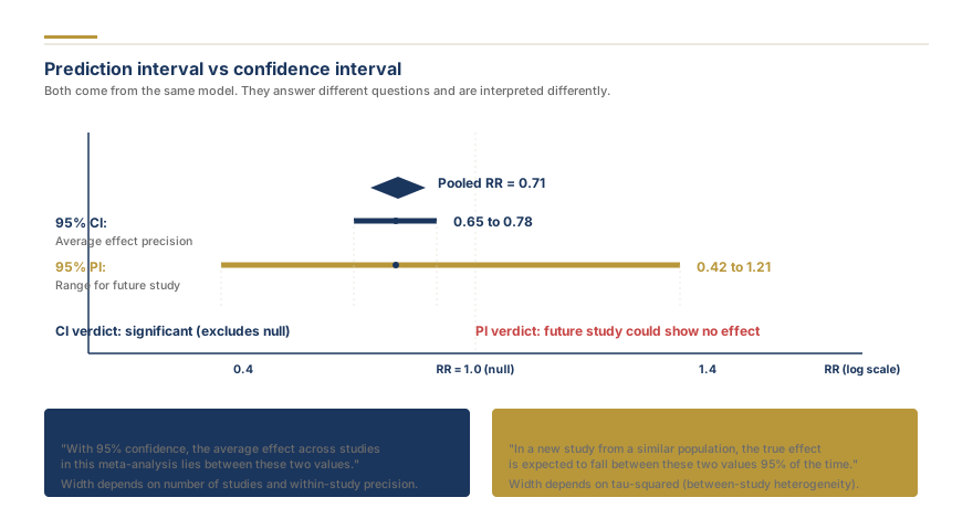
Prediction interval vs confidence interval
The problem with reporting only a pooled effect and its confidence interval in the presence of heterogeneity is that the confidence interval describes only the precision of the average effect across your included studies. It shrinks as you add more studies, regardless of whether the true effects in those studies are converging or diverging.
Consider a pooled risk ratio of 1.35 with a 95% confidence interval of 1.18 to 1.55, p less than 0.001. But if tau-squared is 0.08 and the prediction interval runs from 0.82 to 2.21, the picture is entirely different. In some settings the intervention nearly halves risk; in others it appears harmful. The confidence interval would lead a clinician to apply the intervention universally. The prediction interval correctly signals that the effect is not reliably positive across contexts.
This is precisely the scenario that prompted major journals and the Cochrane Collaboration to recommend reporting prediction intervals whenever I-squared exceeds 0%.
The Mathematics Behind Prediction Intervals
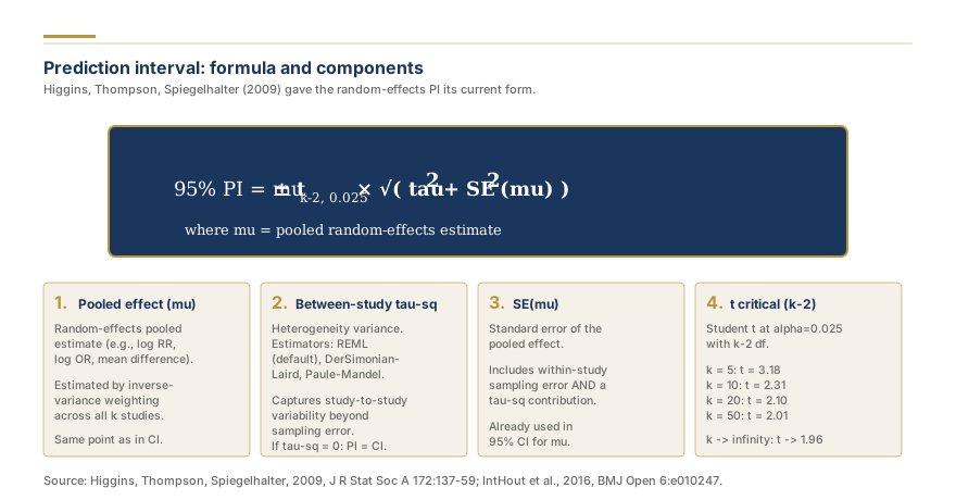
Prediction interval: formula and components
Prediction intervals use the t-distribution with k minus 2 degrees of freedom, where k is the number of studies. The formula is:
PI = pooled estimate +/- t(k-2, 0.975) * sqrt(tau-squared + SE-squared)
The t-distribution accounts for the additional uncertainty introduced by estimating tau-squared from a limited number of studies. When k is small, the t-distribution has heavy tails, and prediction intervals are appropriately wide.
For k equals 5 studies, the t-critical value at alpha 0.05 two-tailed with 3 degrees of freedom is 3.18, compared to 1.96 for the normal distribution. This means prediction intervals from small meta-analyses are substantially wider than a naive normal-approximation calculation would suggest.
Our compute effect size can help you compute the input effect sizes and standard errors needed before constructing prediction intervals.
Interpreting Prediction Intervals in Practice
When the prediction interval excludes the null: The pooled effect is not only statistically significant on average but also expected to be significant in a new study. This is the strongest form of evidence from a random-effects synthesis.
When the prediction interval crosses the null despite a significant pooled effect: The average effect is positive and distinguishable from zero, but in some settings the true effect may be null or negative. The heterogeneity is large enough that you cannot predict with confidence that a new application will replicate the benefit. Subgroup analyses and meta-regression become the scientific priority.
When the prediction interval crosses the null and the pooled effect is also non-significant: The evidence simply does not support a consistent effect.
Pair your prediction interval interpretation with our free sensitivity analysis to check whether removing any single study collapses the heterogeneity and clarifies the prediction interval.
Need help with your meta-analysis?
Our PhD statisticians run complete meta-analyses: effect sizes, forest plots, heterogeneity testing, and publication-ready results sections.
A Worked Prediction Interval Calculation (Step by Step)
The formula only becomes intuitive once you push real numbers through it. Suppose a random-effects meta-analysis of k = 10 trials returns a pooled log risk ratio of M = 0.30 (RR = 1.35), with a standard error of the pooled estimate SE = 0.072 and a between-study variance of tau-squared = 0.08.
Step 1: Compute the confidence interval (for contrast). CI = M +/- 1.96 x SE = 0.30 +/- 1.96 x 0.072 = 0.30 +/- 0.141 = [0.159, 0.441] on the log scale, which exponentiates to RR 1.17 to 1.55. Every value is above 1, so the average effect looks reliably protective.
Step 2: Combine the two variance components. The prediction interval uses the total dispersion of true effects, sqrt(tau-squared + SE-squared) = sqrt(0.08 + 0.072-squared) = sqrt(0.08 + 0.0052) = sqrt(0.0852) = 0.292.
Step 3: Use the t-critical value with k - 2 degrees of freedom. With df = 10 - 2 = 8, t(8, 0.975) = 2.306 (not 1.96). PI = 0.30 +/- 2.306 x 0.292 = 0.30 +/- 0.673 = [-0.373, 0.973], which exponentiates to RR 0.69 to 2.65.
The contrast is the whole point. The confidence interval (1.17 to 1.55) says the average trial benefits. The prediction interval (0.69 to 2.65) crosses 1, so a future trial in a new setting could plausibly show harm. Reporting only the confidence interval would have hidden that.
Why small k widens the interval sharply. Repeat the calculation with only k = 5 studies (df = 3, t = 3.182), holding the dispersion constant: PI = 0.30 +/- 3.182 x 0.292 = 0.30 +/- 0.929 = RR 0.53 to 3.42. Halving the number of studies nearly doubles the interval width, because the t-distribution has heavy tails when df is small. This is also why a prediction interval is unstable, and often not reported, when k is below 3: with df of 1 or 0 the t-value explodes or is undefined.
library(metafor)
res <- rma(yi, vi, data = dat, method = "REML")   # yi = log RR, vi = variances
predict(res, transf = exp)                         # returns pred, ci.lb/ci.ub, pi.lb/pi.ub
The pi.lb and pi.ub columns are your exponentiated prediction interval. Report them next to tau-squared and I-squared so a reader can see that the width is driven by genuine between-study variability, not by a coding choice. The estimator you pick for tau-squared feeds directly into this width, which is why the REML versus DerSimonian-Laird choice matters here too.
When Prediction Intervals Are Most Valuable
Generalizability assessments: When the question is "will it work for my patients in my hospital?", the prediction interval directly addresses the relevant uncertainty.
Guidelines and policy translation: Health technology assessment bodies are beginning to require prediction intervals alongside confidence intervals in submitted meta-analyses.
Informing future research design: A wide prediction interval that crosses the null is evidence for the value of additional research.
Reporting Prediction Intervals Correctly
A complete reporting statement: "The pooled odds ratio was 1.42 (95% CI: 1.18 to 1.71, p less than 0.001; tau-squared = 0.06, I-squared = 47%). The 95% prediction interval ranged from 0.91 to 2.21, indicating that while the average effect across included studies favors the intervention, the true effect in a future similar study could plausibly range from a modest benefit to a modest increase in odds."
Our free forest plot maker displays prediction intervals as extended bars on the forest plot diagram.
Key Takeaways
Prediction intervals define where a new future study's true effect is expected to fall, accounting for both sampling uncertainty and between-study heterogeneity.
Confidence intervals describe only the precision of the pooled average; they narrow as k increases regardless of how inconsistent the true effects are across studies.
The formula uses the t-distribution with k minus 2 degrees of freedom, producing appropriately wider intervals when k is small.
A prediction interval that crosses the null despite a significant pooled effect is a finding, not a problem: it means the average effect is positive but not reliably replicated across all settings.
Prediction intervals are most valuable for generalizability assessment, guideline development, and justifying future research.
Always report prediction intervals alongside tau-squared and I-squared so readers can understand the source of the interval's width.
Prediction intervals apply only to random-effects models; fixed-effects models do not support this concept.
Uncertain whether your pooled effect is robust under a random-effects model? Our full-service meta-analysis delivers prediction intervals, tau-squared diagnostics, and publication-ready forest plots. Get a custom quote.
Frequently Asked Questions
5
The prediction interval requires estimation of two parameters: the pooled mean effect and tau-squared. Each estimated parameter consumes one degree of freedom, leaving k minus 2 for the t-distribution.
With k equals 2, the degrees of freedom for the prediction interval are zero, making the t-distribution undefined and the prediction interval impossible to calculate meaningfully. Meta-analysis of 2 studies is generally discouraged.
No. Prediction intervals quantify the expected range of future true effects given the observed studies, assuming those studies are a representative sample. Publication bias assessment should accompany prediction interval reporting rather than replace it.
Adding studies reduces the standard error of the pooled estimate and improves the precision of tau-squared estimation. However, if the new studies reveal more heterogeneity, the prediction interval can actually widen as evidence accumulates.
When I-squared is very low and tau-squared is near zero, the prediction interval will closely approximate the confidence interval. Reporting it is still good practice for transparency and because most reporting guidelines recommend prediction intervals whenever a random-effects model is used. Need help with your systematic review or meta-analysis? [Get a free quote](/get-a-quote) from our team of PhD researchers.
Share
Found this useful? Share it with your colleagues.
Need help with your meta-analysis?
Our PhD statisticians run complete meta-analyses: effect sizes, forest plots, heterogeneity testing, and publication-ready results sections.
Reading About Meta-Analysis? Our PhD Team Runs Them Every Day.
From data extraction to forest plots, sensitivity analysis, and a journal-ready manuscript. We handle the full meta-analysis so you can focus on your research question.
Our promise: Free re-run of the pooled analysis if reviewers question the estimate or model.
4.9 / 5Quote within a few hoursmetafor R + Cochrane HandbookPhD methodologistConfidential by default
Dr. Sarah Mitchell holds a PhD in Biostatistics from Johns Hopkins Bloomberg School of Public Health and has over 15 years of experience in systematic review methodology and meta-analysis. She has authored or co-authored 40+ peer-reviewed publications in journals including the Journal of Clinical Epidemiology, BMC Medical Research Methodology, and Research Synthesis Methods. A former Cochrane Review Group statistician and current editorial board member of Systematic Reviews, Dr. Mitchell has supervised 200+ evidence synthesis projects across clinical medicine, public health, and social sciences.
Need professional help with your systematic review or meta-analysis? Get a free quote from our team of PhD researchers.
Reading About Meta-Analysis? Our PhD Team Runs Them Every Day.
From data extraction to forest plots, sensitivity analysis, and a journal-ready manuscript. We handle the full meta-analysis so you can focus on your research question.
CHEERS 2022 checklist explained: all 28 items, what changed from CHEERS 2013, and how to report a cost-effectiveness analysis so payers and journals can use it.
SPIRIT 2025 checklist explained: all 34 items by section, what changed from SPIRIT 2013, and how the protocol lines up with CONSORT 2025 when you report the trial.
ARRIVE 2.0 guidelines explained: the Essential 10 and the Recommended Set, what changed from ARRIVE 2010, and the items journals check in animal research reports.