Risk Ratio Explained: Formula, OR vs HR, Regression
Risk ratio is the relative-risk effect size for cohort and trial data. Formula, 2x2 worked example, vs odds ratio and hazard ratio, regression, reporting.
Dr. Sarah Mitchell
May 13, 2026
Key Takeaways
Risk ratio is the ratio of event probabilities in two groups. Computed from a 2x2 table as R1/R0 where R = events/group size. Use for cohort studies and randomized trials, not for case-control studies.
Risk ratio and odds ratio diverge when the outcome is common. The odds ratio is always more extreme than the risk ratio in both directions when outcomes are common (event rate above 10 percent in either group).
Confidence intervals are built on the log scale: SE(log RR) = sqrt(1/a - 1/(a+b) + 1/c - 1/(c+d)). Exponentiate the symmetric log-scale interval to get the asymmetric original-scale interval.
Adjusted risk ratios in observational studies come from log-binomial regression (direct but prone to non-convergence), Poisson with robust variance (always converges), or modified Poisson by Zou 2004 (recommended default for 2026 practice).
Report risk ratio alongside risk difference and number needed to treat to communicate both relative and absolute effects. Reporting only the risk ratio without absolute risks obscures the clinical magnitude of the comparison.
Risk ratio (also called relative risk) is the ratio of the probability of an event in an exposed group to the probability of the same event in a comparison group, computed as the cumulative incidence in the exposed group divided by the cumulative incidence in the unexposed group. It is the effect-size estimator used by cohort studies, randomized controlled trials, and any analysis where the underlying study design produces incidence data rather than odds. This guide covers the definition with notation, the worked computation from a 2x2 table, the confidence interval on the log scale, the interpretation of values above and below 1, the critical distinction between risk ratio and odds ratio, the connection to hazard ratio and risk difference, the regression methods for adjusted risk ratios, and the most common reporting errors that peer reviewers flag in 2026.
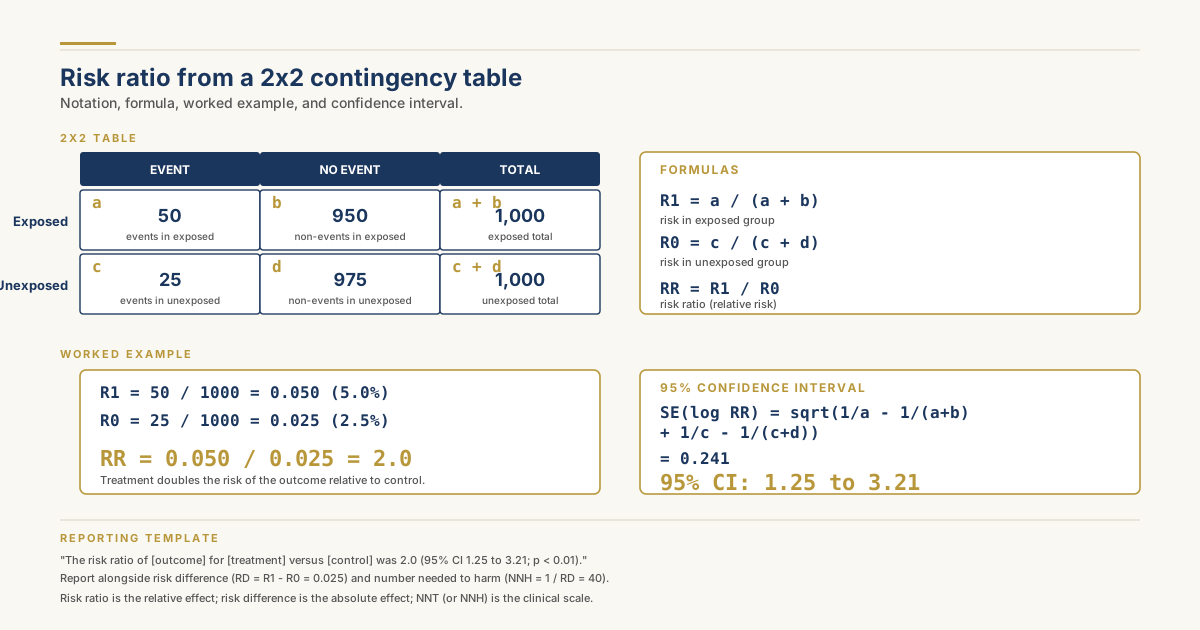
Risk ratio from a 2x2 contingency table: notation, formula, worked example
Risk ratio is one of three closely related effect-size estimators reviewers encounter in binary-outcome analyses: risk ratio, odds ratio, and hazard ratio. The three are not interchangeable. The choice among them is determined by study design, by the timing of outcome assessment, and by whether the outcome is rare or common. A risk ratio reported when an odds ratio was the correct estimator, or vice versa, leads to misinterpretation of the magnitude of effect. The distinction is one of the most-tested concepts in epidemiology examinations and one of the most-corrected errors in peer review.
Risk Ratio Versus Odds Ratio: When Each Estimator Is the Right Choice
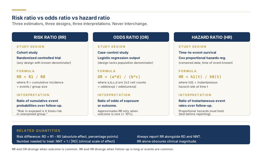
The single most important distinction reviewers must understand is when to use a risk ratio and when to use an odds ratio. The two estimators are mathematically related and numerically similar when the outcome is rare, but they diverge when the outcome is common, and they are produced by different study designs.
Risk ratio requires incidence data. A risk ratio can only be computed when the analyst knows the size of the at-risk population (the denominator of the risk calculation). This is the case in cohort studies, where a known group is followed forward in time, and in randomized controlled trials, where the trial protocol fixes the group size at randomization. In these designs, dividing event counts by group totals gives valid probabilities (the cumulative incidence), and the ratio of those probabilities is the risk ratio.
Odds ratio is required when only sampled cases and controls are available. In a case-control study, the investigator samples a fixed number of cases and a fixed number of controls and asks about exposure status retrospectively. The group denominators are imposed by the design, not by the underlying population, so probabilities (and therefore risks) cannot be computed directly. The odds ratio, which is the ratio of the odds of exposure among cases to the odds of exposure among controls, is the estimator that the design supports. The odds ratio from a case-control study approximates the risk ratio that would have been computed from the equivalent cohort study, but only when the rare-disease assumption holds (the outcome is rare in both exposed and unexposed groups, typically below 10 percent).
When the outcome is common, the odds ratio overestimates the risk ratio. A randomized controlled trial reporting a 50 percent event rate in the control group and a 25 percent event rate in the treatment group has a risk ratio of 0.5 (the treatment halves the risk) but an odds ratio of 0.33 (the odds in the treated group are one third of the odds in the control). The odds ratio is more extreme than the risk ratio in both directions when outcomes are common. Reporting the odds ratio as if it were the risk ratio, or interpreting the magnitude of an odds ratio as if it were a risk ratio, exaggerates the perceived effect. The default in trials with binary outcomes should be the risk ratio; the odds ratio is reported only when a specific reason demands it (e.g., logistic regression was used because of covariate adjustment and a binomial likelihood would not converge).
The two estimators are related by the identity OR = RR × (1 - R0) / (1 - R1), where R0 and R1 are the risks in the two groups. The identity tells you that when R0 and R1 are both small, OR and RR are similar; when they are large, OR is more extreme than RR.
Worked Computation From a 2x2 Table
Consider a randomized trial of 2,000 participants assigned 1:1 to treatment and control. After follow-up, the outcome (a specific adverse event) occurred in 50 of 1,000 treated participants and 25 of 1,000 control participants. The 2x2 table is:
Event
No event
Total
Treatment
50
950
1,000
Control
25
975
1,000
Using the conventional notation a, b, c, d for the four cell counts (a = 50, b = 950, c = 25, d = 975):
Risk in the treatment group: R1 = a / (a + b) = 50 / 1,000 = 0.050 (5.0 percent).
Risk in the control group: R0 = c / (c + d) = 25 / 1,000 = 0.025 (2.5 percent).
Risk ratio: RR = R1 / R0 = 0.050 / 0.025 = 2.0.
The treatment doubles the risk of the adverse event compared to control. Note that the risk difference (a separate but related effect size) is 0.050 - 0.025 = 0.025, or 2.5 percentage points; the risk ratio and risk difference together give the complete picture (the relative and absolute change). The relationship to the effect size calculation for meta-analysis framework is direct: the log risk ratio and its sampling variance are the standard inputs to a random-effects meta-analysis of binary outcomes.
Confidence Interval on the Log Scale
The risk ratio is asymmetric on the original (linear) scale: it can range from 0 to infinity, with 1 as the null. To construct a symmetric confidence interval, the standard approach is to compute the log risk ratio, build a symmetric confidence interval around the log value, and exponentiate back to the original scale. The standard error of the log risk ratio is:
For the worked example: SE(log RR) = sqrt(1/50 - 1/1000 + 1/25 - 1/1000) = sqrt(0.020 - 0.001 + 0.040 - 0.001) = sqrt(0.058) = 0.241.
The log RR is ln(2.0) = 0.693. The 95 percent confidence interval on the log scale is 0.693 plus or minus 1.96 times 0.241, giving (0.221, 1.165). Exponentiating: exp(0.221) = 1.247 and exp(1.165) = 3.205. So the 95 percent confidence interval on the risk ratio is (1.25, 3.21), and because the interval excludes 1.0, the difference is statistically significant at conventional thresholds. The complete derivation and intuition for confidence intervals on the log scale covers why the log transform is necessary and how to read it on a forest plot.
Interpretation: RR = 1, RR > 1, RR < 1
The interpretation of the risk ratio depends on its value relative to the null:
RR = 1.0 (null value). The event probability in the exposed group equals the event probability in the unexposed group. The exposure has no association with the outcome at the population level.
RR > 1.0 (positive association). The exposed group has a higher event probability than the unexposed group. The exposure is a risk factor if the outcome is undesirable. For RR = 1.5 the exposure is associated with a 50 percent relative increase in risk; for RR = 2.0 the risk is doubled; for RR = 3.0 the risk is tripled. The clinically important threshold depends on the baseline risk: doubling a 1 percent risk to 2 percent (RR = 2.0) is a 1 percentage-point absolute increase, while doubling a 30 percent risk to 60 percent is a 30 percentage-point absolute increase. Always report the absolute risk alongside the relative risk for clinical interpretation.
RR < 1.0 (negative association or protective effect). The exposed group has a lower event probability than the unexposed group. For RR = 0.5 the exposure is associated with a 50 percent relative reduction in risk; for RR = 0.8 with a 20 percent reduction. If the exposure is a treatment in a trial and the outcome is undesirable (death, recurrence, adverse event), RR less than 1 indicates a beneficial treatment effect.
The magnitude of RR > 1 versus RR < 1 is asymmetric in interpretation: a risk ratio of 2.0 is the reciprocal of 0.5, so an exposure with RR = 2.0 for the outcome of interest has RR = 0.5 in the mirror-image comparison (swapping the exposed and unexposed groups). When meta-analyzing studies that report RRs in different directions, always re-orient them so the reference direction is consistent across studies.
Risk ratio versus odds ratio versus hazard ratio: study design and interpretation
Need statistical analysis support?
Our PhD statisticians handle data analysis, produce reproducible R code, and write results sections that satisfy peer reviewers.
Risk Ratio Versus Hazard Ratio in Time-to-Event Analysis
The hazard ratio (HR) appears in time-to-event analyses, typically from Cox proportional hazards regression. A hazard ratio is the ratio of the instantaneous hazard (event rate per unit time) in the exposed group to the hazard in the unexposed group, averaged over follow-up time. It is not the same as the risk ratio, and the differences matter for interpretation.
Risk ratio uses cumulative incidence over a fixed follow-up window. A risk ratio of 2.0 over five years of follow-up means that 5-year cumulative event probability is twice as high in the exposed group.
Hazard ratio uses instantaneous rate, independent of total follow-up. A hazard ratio of 2.0 means that at any moment during follow-up, the event rate in the exposed group is twice the event rate in the unexposed group.
For rare events and short follow-up, RR and HR are numerically similar. For common events and long follow-up, HR is more extreme than RR because hazards multiply while risks compound. Reporting an HR from a Cox model and describing it as if it were a risk ratio is a category error; the appropriate language is "the hazard of [event] was X times higher" or "the rate of [event] was X times higher," not "the risk of [event] was X times higher." The hazard ratio also depends on the proportional hazards assumption (the ratio is constant over time), which should be tested before reporting.
Risk Ratio Versus Risk Difference and Number Needed to Treat
The risk difference (RD) is the simple subtraction R1 minus R0. It is the absolute reduction (or increase) in event probability and is the most directly clinically interpretable effect size. For the worked example, RD = 0.025 (2.5 percentage points absolute increase in the adverse event with treatment).
The number needed to treat (NNT) is the reciprocal of the risk difference: NNT = 1 / |RD|. For a beneficial treatment, NNT is the number of patients that must be treated to prevent one bad outcome relative to the control. For the worked example, the treatment is harmful (NNT to harm = 1 / 0.025 = 40, meaning treating 40 patients results in one additional adverse event). The odds ratio and number needed to treat calculator handles the full conversion from any effect size to NNT.
Risk ratio, risk difference, and number needed to treat are three complementary views of the same comparison and should usually be reported together in clinical research. RR captures the relative effect; RD captures the absolute effect; NNT captures the clinical scale of the effect.
Adjusted Risk Ratios in Regression
In observational studies, the unadjusted (crude) risk ratio confounds the exposure effect with other variables. The adjusted risk ratio controls for confounders through a regression model. Three regression approaches produce a risk ratio rather than an odds ratio.
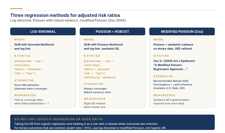
Three regression approaches for adjusted risk ratios: log-binomial, Poisson with robust variance, modified Poisson
Log-binomial regression. A generalized linear model with a binomial likelihood and a log link, which directly parameterizes the risk ratio: exp(beta) = RR. The model often fails to converge when multiple covariates push predicted probabilities above 1.0, which is the boundary of the binomial parameter space. When it does converge, it gives the unbiased risk ratio. In R: glm(outcome ~ exposure + covariates, family = binomial(link = "log")).
Poisson regression with robust variance. A Poisson-likelihood generalized linear model with a log link, applied to binary data. The Poisson model assumes the outcome can range from 0 to infinity, which is wrong for a binary 0/1 outcome, so the model-based standard errors are too large. The fix is to use robust (sandwich) variance estimates, which correct the standard errors back to valid coverage. The Poisson model always converges (no upper-boundary problem) and reports a risk ratio. In R: glm(outcome ~ exposure + covariates, family = poisson(link = "log")) followed by coeftest(model, vcov = sandwich) from the sandwich package.
Modified Poisson regression by Guangyong Zou (2004). A specific algorithmic refinement of Poisson with robust variance, popularized by Zou's 2004 American Journal of Epidemiology paper "A Modified Poisson Regression Approach to Prospective Studies with Binary Data." The Zou method is essentially Poisson with sandwich variance applied to binary outcomes and is now the recommended default for adjusted risk ratios in modern epidemiology. The method is implemented in standard statistical software with a single command (sandwich variance flag).
The historical alternative of taking the odds ratio from a logistic regression and treating it as if it were a risk ratio is biased and should not be done when the outcome is common.
Reporting Risk Ratios in CONSORT and STROBE
For randomized controlled trials, the CONSORT reporting standard requires the trial's primary effect estimate alongside its confidence interval; for binary outcomes this is the risk ratio (or risk difference) with 95 percent CI. The standard text is: "the risk ratio of [outcome] for [treatment] versus [control] was [point estimate] (95 percent CI [lower, upper]; p = [value])." The risk difference and number needed to treat are reported in addition.
For observational cohort studies, the STROBE reporting standard requires the adjusted risk ratio (from log-binomial, modified Poisson, or equivalent) with the list of covariates controlled. The standard text is similar to CONSORT with an additional sentence specifying the regression model and the covariate adjustment.
For case-control studies, STROBE requires the odds ratio (since case-control designs do not support direct risk ratio estimation). The odds ratio is reported with the proviso that it approximates the risk ratio only when the outcome is rare.
For systematic reviews and meta-analyses, the PRISMA 2020 standard requires the pooled risk ratio (or odds ratio if the included studies report odds ratios) with 95 percent CI, alongside heterogeneity statistics (tau-squared, I-squared, Q test) and the prediction interval. The pooled estimate appears on the forest plot for risk ratios at the bottom of the per-study display.
Common Errors Reviewers Make
Three errors account for most peer-review comments on risk-ratio reporting in 2026.
Comparing risk ratios across studies with different baseline risks without noting the absolute effect. A risk ratio of 2.0 looks the same in a study where the baseline risk is 1 percent (treatment risk 2 percent) and in a study where the baseline risk is 30 percent (treatment risk 60 percent). The two studies are profoundly different clinically. Reviewers should always report the absolute risk in each arm alongside the risk ratio, and meta-analyses should examine whether the risk ratio is consistent across studies with different baseline risks (a common reason for heterogeneity).
Reporting an odds ratio as if it were a risk ratio. When the outcome is common, the OR is more extreme than the RR. A randomized trial of a drug for a common condition reporting "the odds ratio for [outcome] was 0.5" without computing the risk ratio overstates the treatment effect. The fix is to compute the risk ratio directly from the cell counts (which a trial always reports) or to use a log-binomial or modified Poisson regression.
Misreading the log scale on a forest plot. Forest plots of risk ratios are typically drawn on a logarithmic x-axis so the null value of 1.0 sits in the middle and a risk ratio of 0.5 is the same visual distance from null as 2.0. Readers who treat the x-axis as linear misinterpret the magnitude of effect. The convention is so universal that visual conventions for the x-axis are treated as the default in modern forest-plot drawing tools.
A fourth, less common, error is transposing the reference group. Reporting "RR = 2.0 favoring treatment" when the calculation actually gave "RR = 2.0 against treatment" inverts the conclusion. The convention is to state the comparison explicitly: "RR = 2.0 (treatment versus control)" with the named groups in the cited order.
Reference Group, Direction, and Why "Relative Risk" Is the Right Plain Language
The term relative risk is interchangeable with risk ratio in clinical and epidemiological practice. Cochrane Handbook chapters use "risk ratio" because it is precise; clinical journals often use "relative risk" because it reads more naturally. They are identical quantities. The plain-language interpretation that most clinicians find intuitive is "the risk in the exposed group is X times the risk in the unexposed group," where X is the relative-risk value.
The direction of comparison must always be explicit. A risk ratio of 0.5 for treatment versus placebo means the treated group has half the risk; a risk ratio of 0.5 for placebo versus treatment means the placebo group has half the risk (i.e., the treatment doubled the risk). The convention in clinical trial reporting is that the experimental arm is the numerator and the comparator is the denominator, but always confirm by checking the cell counts. The full effect size conversion framework between RR, OR, Cohen's d, and Hedges' g covers cross-metric translation when meta-analyzing studies that report different effect sizes.
For epidemiological analyses where the choice of estimator interacts with study design, with confounder adjustment, and with the assumptions of the underlying regression model, biostatistics support for epidemiological analyses provides the methodological scaffolding for the analysis plan and the eventual reporting.
Frequently Asked Questions
What does risk ratio tell us?
Risk ratio tells us how many times more (or less) likely an event is in an exposed group compared to an unexposed group. A risk ratio of 2.0 means the event is twice as likely in the exposed group; a risk ratio of 0.5 means it is half as likely. The risk ratio is a relative effect size, so it should be reported alongside the absolute risk in each group and the risk difference to give a complete clinical picture.
What is the difference between risk ratio and odds ratio?
Risk ratio is the ratio of probabilities; odds ratio is the ratio of odds (odds = p / (1-p)). They are numerically close when the outcome is rare (event rate below 10 percent in both groups) but diverge when the outcome is common. The odds ratio is always more extreme than the risk ratio in both directions when outcomes are common, so reporting an odds ratio as if it were a risk ratio overstates the magnitude of effect. Use risk ratio for cohort studies and trials; use odds ratio for case-control studies where the design forces it.
How do you calculate a risk ratio?
From a 2x2 table with cells a, b, c, d (a = events in exposed, b = non-events in exposed, c = events in unexposed, d = non-events in unexposed): risk in exposed R1 = a/(a+b); risk in unexposed R0 = c/(c+d); risk ratio RR = R1/R0. For example, 50 events in 1,000 treated versus 25 in 1,000 controls gives R1 = 0.05, R0 = 0.025, RR = 2.0. The 95 percent confidence interval is built on the log scale using SE(log RR) = sqrt(1/a - 1/(a+b) + 1/c - 1/(c+d)) and exponentiating the resulting log-scale interval.
What is a good risk ratio?
The interpretation depends on whether the outcome is desirable or undesirable. For an undesirable outcome (death, recurrence, adverse event), a risk ratio below 1.0 favors the exposure (or treatment) and a value above 1.0 indicates harm. For a desirable outcome (cure, response, healing), a risk ratio above 1.0 favors the exposure. Clinical importance also depends on the baseline risk: RR = 2.0 doubling a 1 percent baseline (to 2 percent absolute) is much smaller in clinical impact than RR = 2.0 doubling a 30 percent baseline.
Is risk ratio the same as relative risk?
Yes. Risk ratio and relative risk are the same quantity and are used interchangeably in clinical and epidemiological literature. Some Cochrane methodological writing prefers "risk ratio" because it is unambiguous; many clinical journals prefer "relative risk" because it reads more naturally. The plain-language interpretation is identical: how many times more (or less) likely an event is in the exposed group compared to the unexposed group.
When should I use risk ratio versus hazard ratio?
Use risk ratio when you have cumulative incidence over a defined follow-up period and you want to express the relative cumulative event probability. Use hazard ratio when you have time-to-event data, you have used Cox proportional hazards regression, and you want to express the relative instantaneous event rate (averaged over follow-up). Hazard ratio depends on the proportional hazards assumption (constant ratio over time), which should be tested. RR and HR are numerically similar for rare events and short follow-up, divergent for common events and long follow-up.
Pro Tip
Always report the absolute risk in each arm alongside the risk ratio. A risk ratio of 2.0 doubling a 1 percent baseline (absolute increase 1 percentage point) is profoundly different clinically from doubling a 30 percent baseline (absolute increase 30 percentage points).
Pro Tip
For randomized trials and cohort studies with binary outcomes, default to risk ratio rather than odds ratio. The odds ratio overestimates the magnitude of effect when outcomes are common, leading to overinterpretation.
Pro Tip
Test the proportional hazards assumption before reporting a hazard ratio from Cox regression. Schoenfeld residual tests are standard; if the assumption fails, report time-stratified hazard ratios or use a different model.
Pro Tip
Use modified Poisson regression by Zou (2004) as the default for adjusted risk ratios in observational studies. It always converges and gives valid robust standard errors when implemented with sandwich variance.
Pro Tip
Always orient the direction of comparison explicitly: 'RR = 2.0 (treatment vs control)' is unambiguous; 'RR = 2.0' alone is not. Specify which group is the numerator and which is the denominator at every report.
Frequently Asked Questions
6
Risk ratio tells us how many times more (or less) likely an event is in an exposed group compared to an unexposed group. A risk ratio of 2.0 means the event is twice as likely in the exposed group; a risk ratio of 0.5 means it is half as likely. The risk ratio is a relative effect size, so it should be reported alongside the absolute risk in each group and the risk difference to give a complete clinical picture.
Risk ratio is the ratio of probabilities; odds ratio is the ratio of odds (odds = p / (1-p)). They are numerically close when the outcome is rare (event rate below 10 percent in both groups) but diverge when the outcome is common. The odds ratio is always more extreme than the risk ratio in both directions when outcomes are common, so reporting an odds ratio as if it were a risk ratio overstates the magnitude of effect. Use risk ratio for cohort studies and trials; use odds ratio for case-control studies where the design forces it.
From a 2x2 table with cells a, b, c, d (a = events in exposed, b = non-events in exposed, c = events in unexposed, d = non-events in unexposed): risk in exposed R1 = a/(a+b); risk in unexposed R0 = c/(c+d); risk ratio RR = R1/R0. For example, 50 events in 1,000 treated versus 25 in 1,000 controls gives R1 = 0.05, R0 = 0.025, RR = 2.0. The 95 percent confidence interval is built on the log scale using SE(log RR) = sqrt(1/a - 1/(a+b) + 1/c - 1/(c+d)) and exponentiating the resulting log-scale interval.
The interpretation depends on whether the outcome is desirable or undesirable. For an undesirable outcome (death, recurrence, adverse event), a risk ratio below 1.0 favors the exposure (or treatment) and a value above 1.0 indicates harm. For a desirable outcome (cure, response, healing), a risk ratio above 1.0 favors the exposure. Clinical importance also depends on the baseline risk: RR = 2.0 doubling a 1 percent baseline (to 2 percent absolute) is much smaller in clinical impact than RR = 2.0 doubling a 30 percent baseline.
Yes. Risk ratio and relative risk are the same quantity and are used interchangeably in clinical and epidemiological literature. Some Cochrane methodological writing prefers 'risk ratio' because it is unambiguous; many clinical journals prefer 'relative risk' because it reads more naturally. The plain-language interpretation is identical: how many times more (or less) likely an event is in the exposed group compared to the unexposed group.
Use risk ratio when you have cumulative incidence over a defined follow-up period and you want to express the relative cumulative event probability. Use hazard ratio when you have time-to-event data, you have used Cox proportional hazards regression, and you want to express the relative instantaneous event rate (averaged over follow-up). Hazard ratio depends on the proportional hazards assumption (constant ratio over time), which should be tested. RR and HR are numerically similar for rare events and short follow-up, divergent for common events and long follow-up.
Share
Found this useful? Share it with your colleagues.
Need statistical analysis support?
Our PhD statisticians handle data analysis, produce reproducible R code, and write results sections that satisfy peer reviewers.
Need a Statistician? Our PhD Team Handles the Numbers.
From data cleaning to advanced statistical analysis, reproducible R code, and a results section ready for peer review. We handle the stats so you focus on the science.
Our promise: Free re-run and re-write if reviewers question the analysis or reporting.
4.9 / 5Quote within a few hoursReproducible R or Stata codePhD methodologistConfidential by default
Dr. Sarah Mitchell holds a PhD in Biostatistics from Johns Hopkins Bloomberg School of Public Health and has over 15 years of experience in systematic review methodology and meta-analysis. She has authored or co-authored 40+ peer-reviewed publications in journals including the Journal of Clinical Epidemiology, BMC Medical Research Methodology, and Research Synthesis Methods. A former Cochrane Review Group statistician and current editorial board member of Systematic Reviews, Dr. Mitchell has supervised 200+ evidence synthesis projects across clinical medicine, public health, and social sciences.
Need a Statistician? Our PhD Team Handles the Numbers.
From data cleaning to advanced statistical analysis, reproducible R code, and a results section ready for peer review. We handle the stats so you focus on the science.
Krippendorff's alpha explained: what it measures, how it differs from Cohen's kappa, acceptable thresholds, and which agreement coefficient fits your coding design.
CHEERS 2022 checklist explained: all 28 items, what changed from CHEERS 2013, and how to report a cost-effectiveness analysis so payers and journals can use it.
SPIRIT 2025 checklist explained: all 34 items by section, what changed from SPIRIT 2013, and how the protocol lines up with CONSORT 2025 when you report the trial.