RNA Sequencing Analysis: A Complete Guide to the RNA-seq Pipeline

RNA sequencing analysis turns the raw reads from an RNA-seq experiment into a list of genes that change between your conditions, with the statistics to defend it. The sequencer hands you millions of short reads in FASTQ files; RNA-seq analysis is everything that happens next, from quality control through alignment and quantification to differential expression and pathway interpretation. This guide walks the full pipeline, names the tools at each step, and explains how to read and report the output.

If you have FASTQ files and need to know which genes responded to a treatment, or a reviewer has asked for a re-analysis your lab cannot run, this guide shows you what a complete RNA-seq data analysis looks like and where the decisions that make or break a result actually live.

Why the Design Matters More Than the Aligner

It is tempting to think of RNA-seq analysis as a tool-selection problem: pick the right aligner, pick the right differential expression package, done. In practice the single biggest determinant of whether your result holds up is the experimental design, which is fixed before any read is sequenced. Too few biological replicates, conditions confounded with batch, or RNA quality that varies systematically between groups will sink an analysis no matter how good the software is.

For bulk RNA-seq, three to four biological replicates per group is the practical minimum, and technical replicates do not substitute for biological ones. Samples should be randomized across library preparation and sequencing batches so that the batch effect is not perfectly aligned with the biological effect you care about. Get this right and the rest of the pipeline is a series of well-trodden steps; get it wrong and there is no statistical rescue.

The RNA-seq Analysis Pipeline, Step by Step

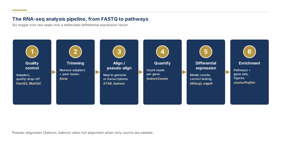
Every RNA-seq pipeline runs through the same backbone. The specific tools vary, but the logic does not.

1. Quality control. Run FastQC on every FASTQ file and aggregate with MultiQC. This single report exposes most problems up front: adapter read-through, per-base quality drop-off, duplication, and unexpected sequence content.
2. Trimming. Remove adapters and low-quality bases with fastp or Trimmomatic, then re-run QC to confirm the trimming worked and did not over-clip.
3. Alignment or pseudo-alignment. Map reads to the reference genome with STAR or HISAT2 when you need a BAM file for visualization or novel-transcript work, or pseudo-align with Salmon or kallisto when you only need gene or transcript counts. Pseudo-alignment is dramatically faster and feeds straight into the next step.
4. Quantification. Produce a count matrix of reads per gene per sample, either from the aligned reads with featureCounts or directly from Salmon.
5. Differential expression. Load the count matrix into DESeq2, edgeR, or limma-voom in R, specify the design formula and the contrasts you care about, and run the test. These packages model the count data correctly and apply multiple-testing correction.
6. Interpretation and enrichment. Translate the gene list into biology with pathway and gene set enrichment analysis, and render volcano plots, heatmaps, and PCA.

For the experimental design and the statistical modeling that sit on top of this pipeline, our statistical modelling support handles complex designs, mixed models, and the multiple-testing decisions that a standard workflow does not cover.

Differential Expression: Where the Answer Lives

The heart of most RNA-seq analysis is differential expression analysis, the test that decides which genes changed. Raw read counts cannot be compared directly because libraries differ in depth and genes differ in length, so packages such as DESeq2 normalize the counts, model the mean-variance relationship of count data with a negative binomial distribution, and shrink unreliable fold-change estimates for low-count genes.

The output is a table with, for each gene, a log2 fold change, a p-value, and an adjusted p-value that controls the false discovery rate across thousands of simultaneous tests. A gene is called differentially expressed when its adjusted p-value sits below your threshold (commonly 0.05) and its fold change is large enough to matter biologically. Reporting raw p-values without correction, or ranking by fold change alone, is one of the most common and most criticized RNA-seq mistakes.

How to Interpret RNA-seq Results

A differential expression table is not the answer; it is the raw material for the answer. Start with the diagnostics. The PCA plot should show your samples separating by condition rather than by batch or sequencing lane; if they cluster by batch, you have a confound to model or, in the worst case, an uninterpretable experiment. The volcano plot then shows the trade-off between effect size and significance at a glance.

From there, validate the biology. Do the top differentially expressed genes make sense for your system? Then move from single genes to processes with pathway and gene set enrichment analysis, which detects coordinated shifts across functionally related genes that individual-gene testing can miss. This is what turns a gene list into a story a reviewer will believe.

Beyond Bulk RNA-seq

Bulk RNA-seq measures average expression across all the cells in a sample, which is the right tool for many designs but blind to cellular heterogeneity. When the question is which cell types are present and how they differ, single-cell RNA-seq analysis resolves expression cell by cell. When the goal is the pathway and network-level view across the whole transcriptome, transcriptomics analysis covers the broader methods. And when you need variants and genome structure rather than expression, genome sequencing analysis is the corresponding DNA workflow.

All of these sit under the same reproducible approach described on our bioinformatics pipeline support page, where the full pipeline is version-pinned and delivered with the command log.

Normalization and the Negative Binomial Model, in Depth

The reason raw counts cannot be compared between samples is that they confound three things: how much a gene is expressed, how deeply the library was sequenced, and how the rest of the transcriptome behaved. A handful of very highly expressed genes can soak up reads and make every other gene look lower in that sample, a problem called composition bias that simple total-count scaling does not fix. DESeq2 corrects it with median-of-ratios size factors: it forms a synthetic reference from the geometric mean of each gene across samples, divides every sample by that reference gene by gene, and takes the median of those ratios as the sample's size factor, a value robust to a few dominating genes. edgeR solves the same problem with TMM (trimmed mean of M-values). This is also why TPM, FPKM, and CPM are the wrong currency for differential expression: they normalize within a sample for gene length or depth and are fine for visualization or reporting an expression level, but they do not correct composition across samples.

The second modeling decision is the distribution. Read counts are not Poisson, because biological replicates vary more than Poisson sampling allows: the variance exceeds the mean, a property called overdispersion. DESeq2 and edgeR therefore fit a negative binomial with a gene-specific dispersion parameter that captures this extra variability. With only three or four replicates each gene's dispersion is estimated very imprecisely, so both packages apply empirical Bayes shrinkage, pooling information across all genes to shrink each gene's dispersion toward a fitted mean-dispersion trend. That borrowing of strength is precisely what makes small-replicate RNA-seq analysable at all. limma-voom takes a different route to the same end: it transforms counts to log2 counts-per-million, estimates the mean-variance relationship and converts it into precision weights, then runs the well-understood linear-model and empirical-Bayes machinery of limma on the weighted data.

The Design Formula Is the Analysis

Almost every consequential decision in RNA-seq lives in the design formula, not the tool. A formula such as ~ batch + condition tells the model to estimate and remove the batch contribution before testing condition, and the contrast you extract names the exact comparison. An additive model assumes the treatment effect is the same in every group; an interaction model such as ~ genotype * treatment adds a term that explicitly tests whether the treatment effect differs between genotypes, which is often the real scientific question. Getting this structure right is what separates a defensible result from a misleading one.

Known nuisance variables (batch, sex, RNA integrity) belong in the model as covariates, never subtracted out beforehand, because subtracting an effect and then testing on the residuals double-uses the data and understates uncertainty. When the unwanted variation is latent (an unrecorded batch, a hidden processing difference), estimate it from the data with surrogate variable analysis (sva) or RUVSeq and add those estimated factors to the design. None of this can rescue a design that confounds batch with condition, where every treated sample sat in one batch and every control in another: that effect is not identifiable by any method, which is why randomization at the bench matters more than any downstream trick. Finally, shrink log fold changes with apeglm or ashr before ranking genes so that low-count genes do not produce huge unreliable fold changes, use independent filtering to drop genes too low to be testable and recover power, and control the false discovery rate with Benjamini-Hochberg. Use a Wald test for a single two-group contrast and a likelihood-ratio test for time courses or multi-level factors.

library(DESeq2)
dds <- DESeqDataSetFromMatrix(countData = counts, colData = meta,
                              design = ~ batch + condition)
dds <- dds[rowSums(counts(dds)) >= 10, ]          # light pre-filter
dds <- DESeq(dds)
res <- results(dds, contrast = c('condition', 'treated', 'control'),
               alpha = 0.05)
library(apeglm)                                    # shrink before ranking
res <- lfcShrink(dds, coef = 'condition_treated_vs_control', type = 'apeglm')

From Counts to a Publication Figure

Once the differential expression result is in hand, the work shifts to presentation: volcano plots, annotated heatmaps, PCA, and enrichment dot plots that meet a journal's figure standards. Our figure preparation service takes the analysis output and produces final, journal-compliant figures, so the result is not just correct but legible to a reviewer.

A complete RNA-seq data analysis ships as a package: a QC report, the reproducible pipeline with every tool version pinned, the count matrix, the differential expression tables, publication-ready figures, and methods text with the exact tools, versions, and parameters ready to paste into your manuscript.

When you are ready, get a free quote with a short description of your design and sample number, or explore the full list of research services to combine RNA-seq with statistics, visualization, or manuscript support.

Free RNA-sequencing analysis tools

You can work through each step of the analysis in the browser: normalize your read counts to CPM, FPKM, or TPM, calculate log2 fold changes between conditions, adjust p-values for the false discovery rate, then build a volcano plot and draw a clustered heatmap of the significant genes. For the full pipeline handled end to end, see the our bioinformatics team.