Single-cell RNA-seq Analysis: From Raw Counts to Cell Types

Single-cell RNA-seq analysis resolves gene expression one cell at a time, revealing the cell types and states that bulk sequencing averages away. Where a bulk experiment reports the mean expression across an entire tissue, scRNA-seq analysis asks which cells are present, how they differ, and which specific populations respond to a treatment or disease. This guide walks the single-cell pipeline, from per-cell quality control through clustering and UMAP to cell-type annotation, and explains how to read the result.

If you have a count matrix from a droplet platform and need it turned into an annotated map of cell types, or a reviewer has asked you to resolve a bulk signal to its cellular source, this guide shows what a complete single-cell data analysis involves and where its unique pitfalls lie.

What Single-cell Resolution Buys You

Bulk RNA-seq measures the average expression of all the cells in a sample. That average is exactly what you want for many designs, but it is blind to composition: a treatment that doubles one rare cell type and halves another can look like no change at all in bulk. Single-cell RNA-seq removes that blind spot by profiling each cell separately, so you can see which populations exist, which are rare, how they relate along a differentiation trajectory, and which of them actually change.

That resolution comes at a cost. The data are sparse, because only a fraction of each cell's messenger RNA is captured, so the matrix is full of zeros. Dissociating tissue into single cells can stress or lose fragile populations. And the analysis carries technical confounders, doublets and ambient RNA, that have no equivalent in bulk work. A good scRNA-seq analysis spends much of its effort controlling those artifacts before any biology is claimed.

The scRNA-seq Analysis Pipeline

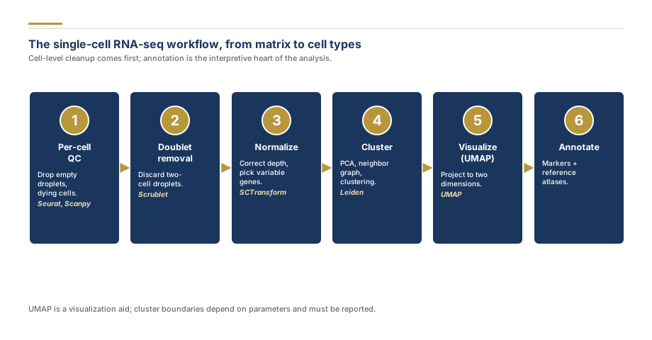
Most single-cell projects run through the same backbone in Seurat (R) or Scanpy (Python). The stages below are near-universal; the parameters at each are where judgment enters.

1. Per-cell quality control. Compute genes per cell, total counts per cell, and mitochondrial fraction, then filter on your own distributions rather than copied tutorial thresholds. High mitochondrial content flags dying cells; very high counts flag likely doublets.
2. Doublet removal. Detect and discard droplets that captured two cells with Scrublet or DoubletFinder, because undetected doublets masquerade as fake intermediate cell states.
3. Normalization and feature selection. Correct for differences in sequencing depth between cells and select the highly variable genes that carry the biological signal.
4. Dimensionality reduction and clustering. Reduce to principal components, build a neighbor graph, and cluster with the Leiden or Louvain algorithm.
5. Visualization. Project the cells to two dimensions with UMAP. Treat this layout as an exploration aid; distances on a UMAP are not quantitatively meaningful.
6. Annotation. Assign each cluster to a cell type using canonical marker genes and, where available, a published reference atlas.

Clustering and UMAP Are Tools, Not Proof

The most common misreading of a single-cell result is to treat the UMAP and its clusters as ground truth. Both depend on choices: the number of principal components, the neighbor count, the clustering resolution. Turn the resolution up and one cluster splits into three; turn it down and three merge into one. None of these is wrong, but the choice must be reported, and cluster boundaries should be validated against biology rather than accepted because the algorithm drew them.

This is why cell type annotation is the interpretive heart of the analysis. A cluster only becomes a cell type when its marker genes match a known population, ideally cross-checked against a reference atlas. Naming clusters by eye, or trusting an automated label without inspecting the markers, is where single-cell stories most often go wrong.

For the statistical side of comparing cell-type proportions or testing within-type differences between conditions, our statistical analysis support handles the compositional and mixed-model methods that these designs require.

How to Interpret Single-cell Results

Interpretation starts with trusting the cleanup. Before reading any biology, confirm that clusters are not driven by technical signal: a cluster defined by mitochondrial genes is dying cells, not a cell type, and a thin bridge between two clusters is often residual doublets. Once the map is clean and annotated, ask the questions that single-cell resolution is uniquely able to answer. Which cell types shift in proportion between your conditions? Within a given cell type, which genes change? Are there rare populations that bulk work would have missed entirely?

The deliverable of a complete single-cell RNA-seq analysis is an annotated UMAP, per-cluster marker tables, differential expression between conditions or cell types, and the reproducible Seurat or Scanpy code with every parameter pinned.

Normalization, Doublets, and Ambient RNA, in Depth

Single-cell counts are sparse unique-molecular-identifier (UMI) tallies in which most genes read zero in any given cell, so the cleanup stage decides whether the biology that follows is real. Three artifacts have no equivalent in bulk work and must each be handled explicitly. Empty droplets are barcodes that captured ambient fluid but no cell; distinguish them from genuine cells with a statistical test on the barcode-rank curve such as EmptyDrops rather than a single hard count cutoff, which discards small real cells and keeps large empty ones. Ambient RNA is cell-free messenger RNA floating in the suspension that contaminates every droplet with a background expression profile; estimate and subtract it with SoupX, DecontX, or CellBender. Doublets are droplets that captured two cells and masquerade as fake intermediate states; Scrublet and DoubletFinder simulate artificial doublets and flag cells whose neighbourhood looks like the simulation.

Normalization is a real modeling choice, not a default. Classic log-normalization scales each cell by its total counts and applies a log transform, which is simple but leaves a residual relationship between sequencing depth and apparent variance. SCTransform instead fits a regularized negative binomial per gene and returns Pearson residuals, a variance-stabilizing transformation that removes the depth-variance coupling and tends to sharpen rare populations. Whichever you choose, set quality thresholds for mitochondrial fraction, gene count, and UMI count from your own data distributions, because a high mitochondrial percentage marks stressed or dying cells and the right cutoff differs by tissue.

Integration and the Statistics of Comparing Populations

When a study spans several donors, runs, or batches, clusters will often form by sample rather than by biology unless you integrate the data. Harmony, Seurat anchor-based integration (CCA or RPCA), and the deep-learning model scVI all align shared cell populations across batches while preserving genuine differences. The danger is over-correction: integrate too aggressively and you erase the very condition effect you came to measure, so always check that a real biological contrast survives integration.

The most consequential and most frequently botched step is testing differences between conditions. Running a per-cell Wilcoxon test across all pooled cells treats thousands of cells from a handful of animals as independent replicates. This is pseudoreplication: it produces vanishingly small p-values that reflect the number of cells, not the number of subjects, and does not replicate. The correct approach is pseudobulk: sum raw counts within each sample and cell type to one profile, then run DESeq2 or edgeR across your true biological replicates exactly as in bulk RNA-seq. Shifts in cell-type proportions between conditions need their own compositional methods, such as scCODA or neighbourhood testing with Milo, because proportions are mathematically constrained to sum to one and are therefore not independent of one another. Cluster resolution, the number of principal components, and the neighbour count all change the cluster count, so report them and validate cluster boundaries against marker biology rather than accepting whatever the algorithm drew.

library(Seurat); library(DESeq2)
# aggregate raw counts to one pseudobulk profile per sample x cell type
pb <- AggregateExpression(seu, group.by = c('sample', 'celltype'),
                          slot = 'counts', return.seurat = FALSE)$RNA
# then build a DESeqDataSet per cell type and test across biological replicates

Where Single-cell Sits in the Wider Workflow

Single-cell RNA-seq is one of several transcriptomic approaches. When cellular resolution is not needed, RNA sequencing analysis on bulk samples is cheaper and simpler. For the pathway and network-level view across the whole transcriptome, transcriptomics analysis covers the broader methods. And for DNA-level questions about variants and genome structure, genome sequencing analysis is the corresponding workflow. All of them run under the reproducible approach described on our bioinformatics analysis support page.

When the annotated result needs to become a journal figure, our publication figure service turns UMAPs, marker dot plots, and proportion bars into final, publication-compliant figures.

Ready to move? Get a free quote with a short description of your platform, cell number, and design, or explore the full list of research services to combine single-cell with statistics, visualization, or manuscript support.

Free tools for exploring single-cell data

Explore the structure of your samples by running a PCA on your data, inspect marker genes across clusters with a clustered expression heatmap, and compare clusters by building a volcano plot after adjusting p-values for the false discovery rate. For a complete analysis, see the managed bioinformatics analysis.